Modern portfolio theory - backbone of portfolio management
Harry Markowitz’s seminal 1952 paper Portfolio Selection remains one of the most frequently cited works in finance, and for good reason. While many books, such as The Intelligent Investor by Graham, already existed, Markowitz was among the first to introduce a rigorous mathematical framework for building and optimizing portfolios.
Portfolio construction matters more than individual assets
What’s pioneering about Markowitz’s work isn’t just the idea of diversification, but the way he mathematically proved that how you combine investments matters just as much, if not more, than the individual assets themselves. His research doesn’t tell you what to invest in but rather how to construct a portfolio that balances risk and return in the most efficient way once you've selected the assets you're interested in. Instead of simply chasing high returns, his framework shifts the focus to optimizing the overall mix, ensuring that the portfolio as a whole is structured to achieve the best possible trade-off between risk and reward.
To reconstruct Markowitz’s Modern Portfolio Theory (MPT) in today's context, we will build an optimal portfolio using two assets: Apple Inc. (AAPL) and Gold (GLD) over a 10-year period. These two assets provide an interesting mix with Apple represents a high-growth, volatile tech stock, while Gold serves as a defensive asset, often moving inversely to equities during market downturns.
Reconstrucing MPT in 2014
Let's assume that in 2014, investor recognizes the future potential growth of two assets:
- Apple (AAPL), a leader in technological innovation.
- Gold (GLD), a traditional safe-haven investment.
Investor constructs two portfolios: one designed for stability (minimum variance) and another focused on growth (maximum risk-adjusted return). But theories are only as good as their real-world performance, so to put their strategy to the test, we'll backtest both portfolios from 2014 to 2024 to see how they actually held up in different market conditions. Crucial aspect of any portfolio analysis is data quality, as the saying goes, "garbage in, garbage out". The accuracy of our results depends entirely on the reliability of our inputs. To ensure meaningful insights, we’ll use monthly returns as our starting point for analysis.
Table 1. Statistics of analyzed assets for years 2004-2014
| Statistic | AAPL | XAUUSD |
|---|---|---|
| Volatility | 37.01% | 19.09% |
| Max Drawdown | -56.91% | -34.03% |
| CAGR | 46.15% | 11.88% |
| Correlation | 0.08 |
All metrics are presented on a yearly basis, except for correlation, which is calculated monthly. Now we'll proceed to find minimum variance portfolio.
Optimized portfolios
Within the framework of Modern Portfolio Theory, the Minimum Variance Portfolio (MVP) is the portfolio that minimizes risk (volatility) for a given set of assets. In contrast, the Tangency Portfolio is the one that achieves the highest risk-adjusted returns, as measured by the Sharpe ratio. While MVP weights can be calculated mathematically, in our case, we can take a more practical approach by simulating multiple portfolios and then identifying both the MVP (the portfolio with the lowest risk) and the optimal risk-adjusted portfolio (the one with the highest Sharpe ratio). We'll achieve this by adjusting the portfolio weights in 10% increments, starting with 100% in GOLD and 0% in AAPL and gradually shifting toward 100% in AAPL and 0% in GOLD, modifying the allocation step by step.
Chart 1. Efficient Frontier with 10% Allocation Increments for years 2004-2014
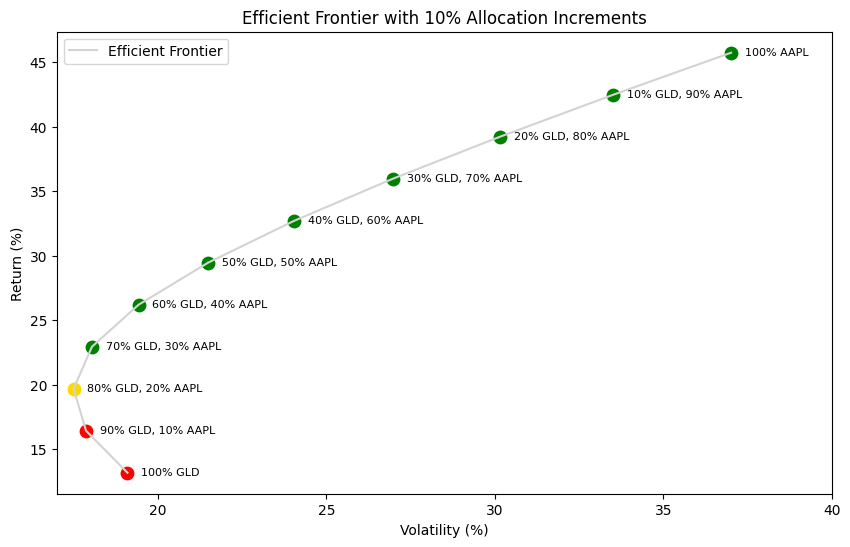
This chart can be divided into three key segments. The first segment coloured as red includes portfolios ranging from 100% GLD / 0% AAPL to 90% GLD / 10% AAPL, which are inefficient. These allocations provide low returns without significantly reducing risk (volatility). A key inefficiency is that for the same level of volatility, investors can achieve higher returns by selecting a different allocation. Even better, shifting to an 80% GLD / 20% AAPL portfolio not only increases returns but also reduces risk (volatility) compared to the 90% GLD / 10% AAPL allocation.
The second segment is the golden dot representing 80% GLD / 20% AAPL portfolio, as it's closest to the Y-axis, indicating its minimal volatility. This is our MVP portfolio, demonstrating its efficiency in terms of volatility. We can see that it doesn't deliver the biggest returns, but it has the lowest possible volatility so we mark it as minimum variance portfolio.
The third segment, represented by green dots, consists of efficient portfolios that offer the best possible returns for a given level of risk. Among these portfolios, we will likely find the one that maximises the Sharpe ratio. To identify the optimal tangency portfolio, we will present a table with the results below.
Table 2. Statistics of simulated portfolios for years 2004-2014
| AAPL Weight (%) | GLD Weight (%) | Return (%) | Volatility (%) | Sharpe Ratio |
|---|---|---|---|---|
| 100.0 | 0.0 | 45.72 | 37.01 | 1.1813 |
| 90.0 | 10.0 | 42.46 | 33.51 | 1.2074 |
| 80.0 | 20.0 | 39.21 | 30.15 | 1.2342 |
| 70.0 | 30.0 | 35.96 | 26.97 | 1.2590 |
| 60.0 | 40.0 | 32.70 | 24.05 | 1.2768 |
| 50.0 | 50.0 | 29.45 | 21.48 | 1.2777 |
| 40.0 | 60.0 | 26.20 | 19.42 | 1.2457 |
| 30.0 | 70.0 | 22.94 | 18.04 | 1.1609 |
| 20.0 | 80.0 | 19.69 | 17.50 | 1.0111 |
| 10.0 | 90.0 | 16.44 | 17.86 | 0.8081 |
| 0.0 | 100.0 | 13.18 | 19.09 | 0.5856 |
The 50% GOLD / 50% AAPL portfolio delivered the highest risk-adjusted returns for the 2004-2014 period with Sharpe ratio equal to 1.2777. However, it was a close call, as the 40% GOLD / 60% AAPL allocation performed nearly as well with Sharpe ratio of 1.2768. Sharpe ratio of 1.2777 mean that for every unit of risk we got 1.2777 units of return over risk free rate. For our calculations we assumed risk free rate to be equal to 2%.
Another key insight from the table above is that while increasing the AAPL allocation leads to higher returns, the rate of return growth diminishes when accounting for risk. Beyond a certain point (the tangency portfolio), any additional return comes with a disproportionately higher level of risk, causing risk-adjusted returns to decline. This effect becomes even more pronounced when leverage is taken into account, but that topic will be explored in a future article.
Backtesting our optimised portfolios even further
As previously mentioned, this modern portfolio construction was based on data from 2004 to 2014. The next step is to extend the backtest to see whether the minimum variance portfolio and tangency portfolio maintain their positions in the following years (2014-2024).
Table 3. Statistics of analyzed assets for years 2014-2024
| Statistic | AAPL | XAUUSD |
|---|---|---|
| Volatility | 27.64% | 14.02% |
| Max Drawdown | -30.46% | -20.01% |
| CAGR | 27.96% | 5.06% |
| Correlation | 0.11 |
As shown in the table above, the correlation between the two assets remains low, even though volatility and CAGR metrics have changed. This suggests that while their individual performance has shifted, their relationship hasn’t strengthened significantly. Now, we'll simulate 2004-2014 portfolios for the years 2014-2024, building on our initial calculations, to see whether the tangency portfolio and the minimum variance portfolio maintain their proportions or if there are shifts in the allocation of the MVP and the optimized portfolio.
Chart 2. Efficient Frontier with 10% Allocation Increments for years 2014-2024
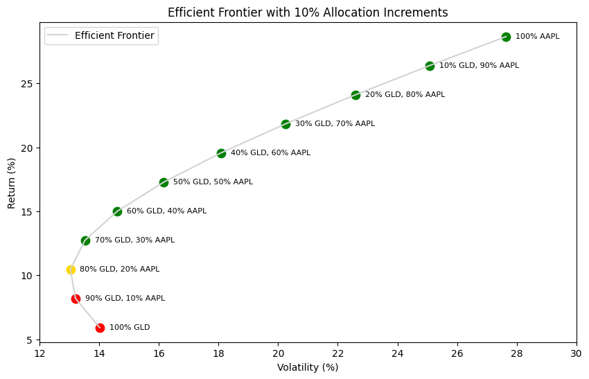
The MVP portfolio maintained its proportions consistently across both periods, 2004-2014 and 2014-2024, comprising 80% GLD and 20% AAPL equity. Additionally, gold-dominant portfolios continued to be suboptimal. In the next step, we'll assess whether the tangency portfolio also retained its proportions over time. The table below presents the risk-adjusted returns, which will help determine whether the tangency portfolio has remained consistent in its allocation.
Table 4. Statistics of simulated portfolios for years 2014-2024
| AAPL Weight (%) | GLD Weight (%) | Return (%) | Volatility (%) | Sharpe Ratio |
|---|---|---|---|---|
| 100.0 | 0.0 | 28.65 | 27.64 | 0.9642 |
| 90.0 | 10.0 | 26.38 | 25.07 | 0.9724 |
| 80.0 | 20.0 | 24.10 | 22.60 | 0.9783 |
| 70.0 | 30.0 | 21.83 | 20.25 | 0.9793 |
| 60.0 | 40.0 | 19.56 | 18.08 | 0.9708 |
| 50.0 | 50.0 | 17.28 | 16.17 | 0.9450 |
| 40.0 | 60.0 | 15.01 | 14.61 | 0.8902 |
| 30.0 | 70.0 | 12.73 | 13.53 | 0.7934 |
| 20.0 | 80.0 | 10.46 | 13.04 | 0.6487 |
| 10.0 | 90.0 | 8.18 | 13.21 | 0.4681 |
| 0.0 | 100.0 | 5.91 | 14.02 | 0.2789 |
Previously, the 50% AAPL / 50% GOLD allocation was identified as the tangency portfolio, delivering the highest risk-adjusted return. However, in the updated backtest, the optimal balance has shifted to 70% AAPL / 30% GOLD, which now holds the highest Sharpe ratio of 0.9793. This change reflects how asset performance and risk characteristics evolve over time, altering the most efficient portfolio composition.
The minimum variance portfolio (MVP) remains unchanged at 20% AAPL / 80% GOLD, but the ideal mix for maximizing risk-adjusted returns now favors a more equity-heavy allocation. Even though the proportions have changed, the Sharpe ratio remains highest in this region, particularly between 60% AAPL / 40% GOLD and 80% AAPL / 20% GOLD, reinforcing that a well-diversified balance between AAPL and GOLD continues to offer the best trade-off between risk and return.
Although historical data cannot guarantee future performance, it remains the best tool available for making informed investment decisions. Sticking rigidly to an optimized portfolio may not always be the best approach, as future conditions are unpredictable. Instead, these optimized allocations should be seen as a guideline and a strong starting point for constructing an efficient portfolio.
TLDR;
- MPT is about combining assets, not stock-picking, to optimize risk and return.
- Efficient Frontier: The best portfolios balancing risk vs. return.
- Minimum Variance Portfolio (MVP): Lowest risk portfolio.
- Tangency Portfolio: Best risk-adjusted return (highest Sharpe ratio).
- MPT is good starting point for portfolio construction and understanding risk-return trade-offs.
All materials are available as Jupyter notebooks in my GitHub repository.
Member discussion